



Traditional relational database management systems (RDBMS) are struggling to handle the scale and complexity of modern data. Google Cloud’s BigQuery, a fully managed, serverless data warehouse, offers a powerful and scalable solution to this challenge. In this blog post, we’ll delve into the advantages of transitioning from legacy RDBMS to a cloud-native data warehouse like BigQuery. We’ll explore how BigQuery’s unique architecture and capabilities, particularly its columnar storage, empower organisations to efficiently extract valuable insights from their data.
A key focus of our discussion will be BigQuery performance optimisation. In the first article from the 2-part series, we will compare the use of normalised and denormalised data storage formats within BigQuery and examine the strengths and weaknesses of each approach. By understanding these nuances, you can make informed decisions about how best to leverage BigQuery’s capabilities for your specific data analytics needs. In part two, we look into optimising the data warehouse with nested fields.
Normalised vs Denormalised Data
Data normalization is a standard practice in traditional relational database management systems (RDBMS). It enhances data organisation and saves storage space through efficient data representation. However, in data warehouses, denormalisation is often preferred. Contrary to typical database practices, this approach allows duplicate field values within a column. While this flattened data structure occupies more storage, its non-relational organisation improves query efficiency. This is achieved through parallel processing using columnar storage, which reduces the need for costly joins.
Not All Queries Benefit from Denormalised Data
Queries that involve grouping by a column with a 1-to-many relationship can face challenges with denormalised data. Grouping necessitates data shuffling, which often involves transferring data across networks between servers or systems. This shuffling process can be slow. Fortunately, BigQuery offers a solution to this issue through the use of nested and repeated fields.
To leverage the tradeoffs between normalised and denormalised data, Google provides the following guidelines:
- Instead of joins, take advantage of nested and repeated fields in denormalized tables.
- Keep a dimension table smaller than 10 gigabytes normalised unless the table rarely goes through UPDATE and DELETE operations.
- Denormalise a dimension table larger than 10 gigabytes unless data manipulation or costs outweigh the benefits of optimal queries.
Query Performance Testing: Normalisation vs Denormalisation
To understand the advantages and disadvantages of using normalised versus denormalised tables for BigQuery performance optimisation, I conducted an experiment using the public dataset table github_repos.commits in BigQuery. The focus was on the columns Commit, Subject, Author_email, and Author_name, which provide metadata about individual commits, including the subject of each commit and information about the author.
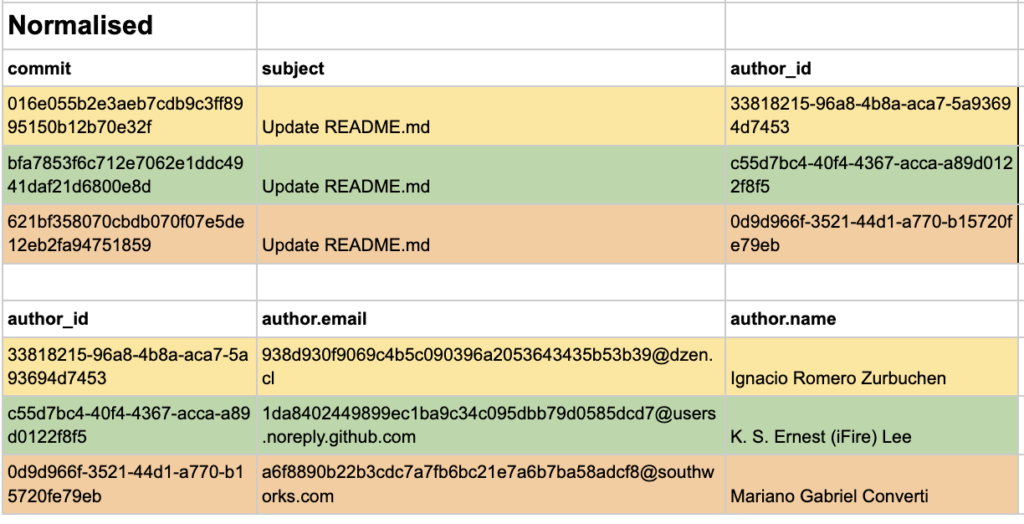
In the original dataset, all columns are stored in the same table, representing a denormalised form. For the experiment, the relevant columns were isolated and also stored in a normalised form. This involved splitting the commit data and author data into two separate tables linked by a unique Author_ID.
The storage requirements for the two scenarios differ significantly. The denormalised table occupies 38.59 GB, whereas the normalised tables use only 31.51 GB combined. This illustrates the storage efficiency achieved through normalisation by eliminating the duplication of author data across multiple tables.
This size discrepancy directly impacts storage costs. In the US multi-region used for testing, the monthly storage cost of the denormalised table is $0.52, while the normalised tables cost $0.39.
The tables have the following formats:

Test Scenarios
To compare the different storage formats, they were tested in three different scenarios and compared based on their query speed and query cost. The specific queries used in the analysis can be found in the appendix.
The three scenarios tested were:
Scenario 1: Finding commit details for a specific author
- This scenario tests the retrieval speed of related data across multiple tables (join performance in normalized vs. single table scan in denormalized).
Scenario 2: Counting Commits per Author
- This scenario tests the performance of aggregation with and without joins (grouping and counting in both normalized and denormalized structures).
Scenario 3: Finding Authors with “Research” in the Name
- This scenario tests the retrieval speed of data from a single table (no joins in either structure but different column sizes due to duplication in denormalized structures)
Test Results
Query Speed
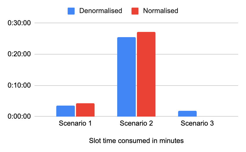
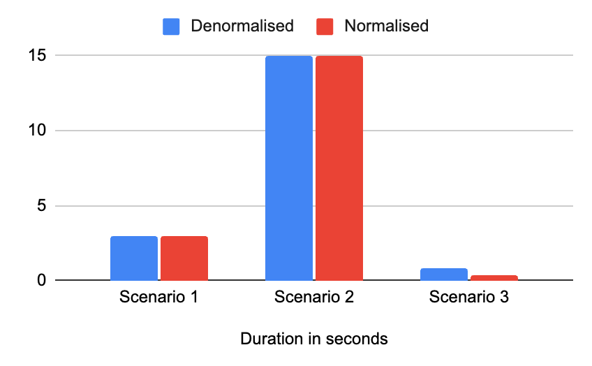
The charts demonstrate that the denormalised format offers superior performance when dealing with data involving both commits and authors. This advantage stems from the elimination of expensive joins between the commit and author tables, which are necessary in the normalized form. Queries of normalised data are often slower for complex queries involving multiple joins, especially if not optimized. BigQuery’s query optimizer can handle joins efficiently, but complex joins can still add overhead.
However, in scenario 3, where the query focuses solely on the uniquely stored authors in the normalised form, the performance of the normalised form significantly surpasses that of the denormalised form. While the cost of joins offsets this advantage in scenarios 1 and 2, scenario 3 does not require any joins, allowing the normalised form’s optimisation to shine.
Although normalised tables offer impressive performance in isolated scenarios, real-world analytics rarely involve analysing a single table. The true value lies in connecting disparate data sources to uncover patterns and relationships. Achieving this with normalised tables necessitates numerous costly joins that significantly slow down query performance.
Currently, billing is based solely on bytes processed, which slightly favours the normalised form. However, this is likely to change as Google plans to incorporate slot time consumed into the billing formula. This change will make the performance differences between normalised and denormalised tables highly relevant to all users and further encourage the adoption of denormalised tables.
Query Cost
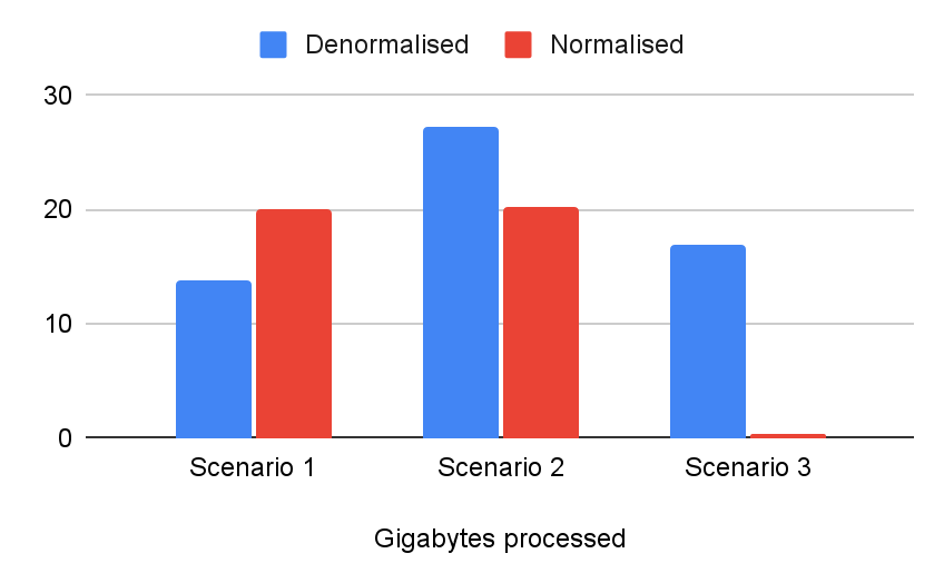
The chart below shows that the bytes processed vary greatly across the three scenarios. Because BigQuery is a columnar storage, the bytes processed and, therefore, query cost only include the columns selected in the query. This greatly reduces cost when only certain columns are of interest.
The results vary based on which columns are part of the query and, in the case of the normalised data, which tables were used and which direction tables were joined.
The query cost of normalised data can be higher for complex queries due to join operations and the amount of data scanned. In contrast, denormalised data often has lower query costs for common analytical queries as less data needs to be scanned and fewer joins are required. This is a key driver for denormalisation in BigQuery.
This can be seen in Scenario 1, where all commit rows have to be scanned in addition to the author table due to the join. In real-world analytics, this will be a frequent occurrence, highlighting the inefficiencies of this approach.
Scenarios 2 and 3 are less costly for normalised data. This is because they are focussed on the smaller author table and, therefore, reduce or even avoid reading the many columns of the commit table. In these simplified test scenarios, it could look like queries on normalised data require less processing. Especially when looking at Scenario 3, which shows a considerable difference in bytes processed. It should however be considered that in most analytics use cases, simple scenarios like these rarely happen.
Query Design
When looking at the queries for the different scenarios, it is easy to see that querying a single table is much easier for the data engineer writing it. This is because denormalised data strongly reduces the need for joins between tables, which speeds up the design of complex queries and makes them much easier to troubleshoot in case something goes wrong.
The Verdict
This analysis highlights the trade-offs between normalised and denormalised data models. Denormalisation can significantly improve the performance and cost of queries involving multiple related entities by eliminating joins. However, this comes at the cost of storage efficiency.
BigQuery’s columnar storage and parallel processing capabilities play a crucial role in efficiently handling both normalised and denormalised data. Its architecture enables it to leverage the strengths of each model, providing flexibility for different query patterns and data access requirements.
Additionally BigQuery offers functionality that combines the best of both normalised and denormalised data models – nested and repeated fields. By leveraging these, BigQuery allows its users to avoid costly joins while keeping the duplication of fields to a minimum. To find out more about these functionalities and how they perform in praxis, stay tuned for part two of this series.
| Feature | Normalised Data | Denormalised Data |
|---|---|---|
| Data Organisation | Data is split into multiple related tables, avoiding redundancy. | Data is stored into fewer tables, with potential duplication of values. |
| Storage Cost | Generally requires less storage space due to reduced redundancy. | May require more storage space due to data duplication. BigQuery’s compression can reduce the actual storage used. |
| Query Performance | Can be slower for complex queries involving multiple joins to retrieve related data. | Generally faster for queries involving multiple related entities. |
| Query Cost | Can be more cost-efficient due to less redundant data being processed, but joining from a larger table can lead to higher query costs. | Lower query costs for common analytical queries as less data needs to be scanned and fewer joins are required. |
| Data Manipulation | More complex updates as changes need to be propagated across multiple tables to maintain consistency. Requires careful management of transactions. | Simpler updates for individual records, but increased risk of data inconsistency if updates are not carefully managed. |
| Use Cases | Suited for when data manipulation or costs outweigh benefits of optimal queries and when a dimension table is smaller than 10 GB, and rarely goes through UPDATE and DELETE operations. | Favoured for analytics and data warehouses where query speed is a priority, particularly when tables are larger than 10 GB and when data manipulation is less frequent. |
| Joins | Requires joins to combine data from multiple tables for analysis. Can involve many joins for complex queries. | Fewer joins required. Often, the data needed is already in a single table. |
| Developer Experience | Data is stored in fewer tables, with potential duplication of values. | Simpler to write queries, especially for analytical use cases. Data exploration and prototyping can be faster. |
Additional resources
Here are some further articles on BigQuery optimisation:
- Part 2 of the BigQuery optimisation series: BigQuery Nested and Repeated Fields
- BigQuery cost optimisation in practice: How Bambuser optimised their BigQuery costs
- BigQuery pricing: How to Prepare for Upcoming Billing Changes

Want to optimise your data warehouse for peak performance?
Contact our Google Cloud experts and unlock the full potential of your data! Hungry for more tech knowledge? Check our Data resources!
Appendix
1. Create Tables
Denormalised data:
CREATE OR REPLACE TABLE `query_speed_blog.git_commits_denormalised` AS (
SELECT
commit,
subject,
STRUCT(
author.email AS email,
author.name AS name
) AS author
FROM
`bigquery-public-data.github_repos.commits`
);
Normalised data:
— Create table for authors with a unique identifier for each author
CREATE OR REPLACE TABLE `query_speed_blog.git_authors_normalised` AS
SELECT
GENERATE_UUID() AS author_id, — Generate a unique ID for each author
author.email AS author_email,
author.name AS author_name
FROM
`query_speed_blog.git_commits_denormalised`
GROUP BY
author_email,
author_name;
— Create table for commits with reference to author
CREATE OR REPLACE TABLE `query_speed_blog.git_commits_normalised` AS
SELECT
t1.commit,
t1.subject,
t2.author_id
FROM
`query_speed_blog.git_commits_denormalised` AS t1
INNER JOIN `query_speed_blog.git_authors_normalised` AS t2 ON t1.author.email = t2.author_email
AND t1.author.name = t2.author_name;
2. Testing Queries
Scenario 1: Finding Commit Details for a Specific Author
Normalised Query
SELECT
c.commit, a.author_name
FROM
`query_speed_blog.git_commits_normalised` AS c
INNER JOIN `query_speed_blog.git_authors_normalised` AS a ON c.author_id = a.author_id
WHERE a.author_name = ‘root’;
Denormalised Query
SELECT
commit, author.name
FROM
`query_speed_blog.git_commits_denormalised`
WHERE author.name = ‘root’;
Scenario 2: Counting Commits per Author
Normalised Query
SELECT
a.author_email,
a.author_name,
COUNT(c.commit) AS commit_count
FROM
`query_speed_blog.git_authors_normalised` AS a
LEFT JOIN `query_speed_blog.git_commits_normalised` AS c ON a.author_id = c.author_id
GROUP BY a.author_email, a.author_name;
Denormalised Query
SELECT
author.email,
author.name,
COUNT(commit) AS commit_count,
FROM
`query_speed_blog.git_commits_denormalised`
GROUP BY author.email, author.name;
Scenario 3: Finding Authors with “Research” in the Name
Normalised Query
SELECT
author_email, author_name
FROM
`query_speed_blog.git_authors_normalised`
WHERE author_name LIKE ‘%Research%’;
Denormalised Query
SELECT
author.email, author.name
FROM
`query_speed_blog.git_commits_denormalised`
WHERE author.name LIKE ‘%Research%’
GROUP BY author.email, author.name;