From SQL to AI: How BigQuery ML Revolutionises the Data Workflow

Estimated reading time: 8 minutes

Building ML models shouldn’t require extracting data, configuring environments, and stitching together half a dozen tools. In reality, the traditional Python workflow is precisely reliant on these aspects: setup, distinct libraries, and nuanced model deployment. However, if one’s data already resides in BigQuery, as it does for many organisations, BigQuery ML enables model development directly within the warehouse. This raises the central question addressed in this article: How does this in-warehouse development compare to traditional approaches? 

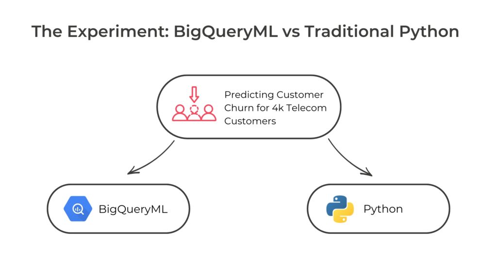
In this article, we will compare BigQuery ML to the traditional Python workflow by building a customer churn model in both environments. We will see the pros and cons of each approach, testing how BQML streamlines preprocessing and deployment. Wondering if you should trade the granular control of Python for the speed and accessibility of SQL-based machine learning? Here are the answers (with some code)!

Predicting Customer Churn: The Two Ways

We’ll compare both approaches using a public telecom dataset with approximately 4,000 customers. The task: predict customer churn (whether someone cancels their service) based on usage patterns, region, and account information. Both approaches will split data into training and testing sets to evaluate model performance on unseen data.

Path A: BigQuery ML

Creating a model in BigQuery ML is deceptively simple, as it abstracts away most of the complexity and overhead, much like other managed cloud solutions. BigQuery ML automatically handles NULL values, splits data for training and evaluation, and in this case, it performs one-hot-encoding for us. Our dataset contains a ‘state’ column with categorical values like NY or WA. BigQuery ML converts these strings into distinct features that the model can process.

With data prep handled, model creation is as simple as selecting an architecture and specifying the target variable (churn: yes or no). While not strictly necessary, excluding redundant or irrelevant variables is a sensible and standard approach; this is done through an except statement.

CREATE MODEL `project.dataset.model_name`
OPTIONS (
  model_type = "LOGISTIC_REG",
  input_label_cols = ["churn"] --target variable
) AS
SELECT
  * EXCEPT (
      customer_id,
      total_day_charge,
      total_eve_charge,
      total_night_charge,
      total_intl_charge
    )
FROM `project.dataset.table_name`

Evaluation on the test set (unseen data) is done with the following structure.

SELECT
  *
FROM ML.EVALUATE (MODEL `project.dataset.model_name`)

This simple approach yields a model that performs quite badly. In this case, the distribution of churn isn’t proportional; roughly 85% of customers don’t churn, so the model defaults to predicting “no churn” for everyone. We can force the model to weigh these equally by adding auto_class_weights = True to the options.

This gives us a slight improvement, but logistic regression seems to hit a ceiling here. Switching to a more powerful architecture is as straightforward as changing "LOGISTIC_REG" to "BOOSTED_TREE_CLASSIFIER". This finally yields a model with satisfactory performance. 

The key takeaway? Iterating requires minimal code changes; you’re working in SQL the entire time, while BigQuery ML does a lot behind the scenes. Train/test splits, one-hot-encoding, and even the scaling of numerical features (a standard approach for logistic regression), all of these common practices that would require explicit implementation in traditional workflows are automatically handled. Let’s see how this compares to the traditional route.

Path B: Python and the rest of the stack

The traditional approach starts with setup, if running locally it is necessary to install Python and the relevant libraries. This is abstracted away if one uses managed environments such as Google Colab or Workbench.

Next, one needs to move data from BigQuery to the development environment. This can either be done manually (exporting and then loading) or by directly querying from Python, which requires proper authentication. The following snippet uses a service account JSON key.

from google.cloud import bigquery
import pandas as pd
import os


#set environment through JSON key and start client
os.environ["GOOGLE_APPLICATION_CREDENTIALS"]="path_to_key.json"
client = bigquery.Client(project="project")
query = '''
SELECT
  * EXCEPT (
      customer_id,
      total_day_charge,
      total_eve_charge,
      total_night_charge,
      total_intl_charge
    )
FROM `project.dataset.table_name`
'''


df = client.query(query).to_dataframe()

We used a query that mimics our BQML EXCEPT statement to avoid loading the full table. Unlike BigQuery ML, the traditional workflow requires most actions to be explicit: handling NULL values (this dataset has none, but typically you’d use pandas to drop or impute them), splitting train/test sets, encoding categorical variables, and scaling numerical features.

All of this is managed by BigQuery ML without being instructed to do so; in Python, the entire preprocessing pipeline is explicit.

from sklearn.model_selection import train_test_split
from sklearn.preprocessing import OneHotEncoder, StandardScaler
from sklearn.compose import ColumnTransformer, make_column_selector
from sklearn.linear_model import LogisticRegression
from sklearn.pipeline import Pipeline
from sklearn.metrics import f1_score
import numpy as np


#separate features and target variables and split sets
y = df["churn"]
X = df.drop(columns=["churn"])


X_train, X_test, y_train, y_test = train_test_split(X, y, test_size=0.2)


#pre process categorical features and scale numerical variables
categorical_transformer = OneHotEncoder(handle_unknown="ignore")
numeric_transformer = StandardScaler()


preprocessor = ColumnTransformer(
    transformers = [
      ("num", numeric_transformer, make_column_selector(dtype_include=np.number)),
      ("cat", categorical_transformer, make_column_selector(dtype_include=object)),
      ("bool", "passthrough", make_column_selector(dtype_include=bool))
    ])


#model pipeline and evaluation
model_pipeline = Pipeline(steps=[
    ("preprocessor", preprocessor),
    ("classifier", LogisticRegression())
])


model_pipeline.fit(X_train,y_train)
y_pred = model_pipeline.predict(X_test)
f1 = f1_score(y_test, y_pred)
print(f"F1-Score: {f1}")

This implementation is much more verbose than BigQuery ML. It yields an F1-score around 0.2. To address class imbalance, we can add class_weight=’balanced’ to the model call, which improves performance to around 0.5. The values are not exact due to the nature of the random shuffling, yet they align with our BigQuery ML results. Interestingly enough, training was nearly instantaneous in Python.

Switching to a boosted tree requires additional adjustments. Tree models don’t benefit from the scaling of features we had applied, and XGBoost’s class weights need to be calculated manually, unlike the previous implementation in scikit-learn.

from xgboost import XGBClassifier


scale_pos_weight = (y_train == False).sum() / (y_train == True).sum()
model_pipeline = Pipeline(steps=[
    ("preprocessor", preprocessor),
    ("classifier", XGBClassifier(scale_pos_weight=scale_pos_weight))
])

This yields an F1-score around 0.8, again with a near-instantaneous training time. While Python offers speed on small datasets, the workflow requires significantly more domain knowledge.

The Takeaway

Differences are stark. BigQuery ML abstracts away the complexity that would otherwise require manual work: no data movement, seamless model switching, and automated data preparation.

BigQuery ML empowers analysts with rapid prototyping. It’s not designed for data scientists who need the full granularity Python allows. For teams without deep ML expertise, the tradeoff makes sense. The underlying mathematics remain consistent; a logistic regression performs the same regardless of implementation.

What about Scale?

On our small dataset, Python’s training speed was faster. But what happens when data grows?

We benchmarked this on a bigger dataset, just shy of 3GB, roughly 10,000 times larger than the original. The BigQuery ML workflow remained identical. Logistic regression training took a few minutes, but the process was unchanged.

However, the Python environment crashed. The likely culprit would be the categorical encoding with more unique values, which exhausted available memory. This is fixable by allocating more RAM, optimising processing with Dask or Polars, switching to distributed Spark clusters, or even sampling the data. The point here is that each solution adds complexity, moving further away from a simple repeatable workflow.

The key insight is that BigQuery ML scales without friction. The same SQL query that worked on 4,000 rows also works on 50 million. No code changes, no architectural rewrites, no infrastructure decisions. BigQuery ML simply works.

What about inference?

Training is only half of the story. In our Python example, to actually use the model, one needs to wrap the code in an API (such as Flask or FastAPI), containerise it with Docker, and then deploy it to a callable endpoint through Google Cloud Run or Kubernetes.

With BigQuery ML, this entire process is skipped. For real-time predictions, adding model_registry = "vertex_ai" to the SQL options automatically exports the model to Vertex AI, where it can be directly deployed as a REST endpoint. No API development, no containerisation, just a single line of code.

Overall comparison:

Bringing all the results together, the trade-offs become clear in a side-by-side comparison, as the true cost of each path is revealed when factoring in developer time, scalability, and deployment overhead.

Dataset	Model	BQML F1 Score	BQML Time	Python F1 Score	Python Time
Small (4k rows)	Logistic Reg. with class weight	0.517	30 sec	~0.5	~Instant
Small (4k rows)	Boosted Tree with class weights	0.789	6 min 38 sec	~0.8	~Instant
Big (~3GB)	Logreg	0.975	2 min 11 sec	Failed	Failed

Python results (~) are approximate due to the random train/test split.

BigQuery ML vs Python: What should you choose?

So which path should you choose? Unfortunately, the answer is the one that nobody likes – it depends. But the table below should help you make an informed decision.

BigQuery ML	Traditional Python
Effortless Scalability: The same SQL query scales from a few to millions of rows with no changes.	Scaling Friction: Requires specific implementation for large datasets (e.g., re-architecting with Spark/Dask).
Zero-Friction Workflow: Lives in the warehouse. No data movement and no setup.	High-Overhead Workflow: Requires data movement and environment setup.
Automated Preprocessing: Handles preprocessing steps automatically (e.g., one-hot encoding, feature scaling, NULLs).	Explicit Preprocessing: You must manually code every step (e.g., StandardScaler, OneHotEncoder).
Simple Deployment: A single SQL command (model_registry) deploys the model to a Vertex AI endpoint.	Nuanced Deployment: Requires building an API (Flask), containerising (Docker), and deploying to infrastructure (Cloud Run).
Less Granularity: Limited to BQML’s supported model architectures.	Total Granularity: Unmatched flexibility for custom architectures (e.g., custom neural networks) and fine-tuning.

When not to use BQML

While BQML handles the vast majority of tabular ML use cases natively, it is bound to pre-defined model architectures. It does not support defining custom neural network layers, which are often employed in specialised applications such as image processing. Since BQML does not currently provide these operations, the Python path remains relevant due to its unmatched flexibility.

Closing remarks

Ultimately, BigQuery ML is about accessibility. It abstracts away the heavy lifting, allowing teams to focus on insights rather than setup, development and deployment. 

For the vast majority of business use cases, the trade-off is overwhelmingly positive: you gain a massive reduction in complexity and time-to-value, losing only the granular control that most standard predictive tasks never actually require.

Looking to optimise your BigQuery data warehouse? We prepared two articles explaining how to do it with nested fields and denormalisation.